Translation Graphs from GrAF/XML files
In this tutorial we will demonstrate how to extract a translation graph from data in digitized dictionaries. The translation graph connects entries in dictionaries, via annotation for “heads” and “translations” within the dictionary. We will demonstrate how to visualize this data with a plotting library and how to export parts of the graph to JSON for interactive visualizations in the web.
You can download this tutorial as IPython notebook here:
https://github.com/cidles/graf-python/blob/master/examples/Translation%20Graph%20from%20GrAF.ipynb
Or as a Python script here:
https://github.com/cidles/graf-python/blob/master/examples/Translation%20Graph%20from%20GrAF.py
Data
For this tutorial we will use data from the project “Quantitative Historical Linguistics”. The website of the project provides a ZIP package of GrAF/XML files for the printed sources that were digitized within the project:
http://www.quanthistling.info/data/downloads/xml/data.zip
The ZIP package contains several files encoded as described in the ISO standard 24612 “Linguistic annotation framework (LAF)”. The QuantHistLing data contains dictionary and wordlist sources. Those were first tokenized into entries, for each entry you will find annotations for at least the head word(s) (“head” annotation) and translation(s) (“translation” annotation) in the case of dictionaries. We will only use the dictionaries of the “Witotoan” component in this tutorial. The ZIP package also contains a CSV file “sources.csv” that contains some information for each source, for example the languages as ISO codes, type of source, etc. Be aware that the ZIP package contains a filtered version of the sources: only entries that contain a Spanish stem that is included in the Spanish swadesh list are included in the download package.
For a simple example how to parse one of the source please see here:
http://graf-python.readthedocs.org/en/latest/Querying%20GrAF%20graphs.html
What are translation graphs?
In our case, translation graphs are graphs that connect all spanish translation with every head word that we find for each translation in our sources. The idea is that spanish is some kind of interlingua in our case: if a string of a spanish translation in one source matches a string in another source this will only be ‘’‘one’‘’ node in our graph. For the head words, this is not the case: matching strings in head words in different source are different nodes in the graph. This holds even if the different sources describe the same language, as different sources will use different orthographies.
To fullfil that need, head words are internally represented as a string with two parts: the head word and its source. Both parts are seperated by a pipe symbol “|”. For example, in a DOT file such a node looks like this:
“ócáji|thiesen1998” [lang=boa, source=thiesen1998_25_339];
The square brackets contain additional attributes here. These attributes are not part of the node’s name, they contain just additonal information the user wants to store with the nodes.
In comparison, a spanish translation looks like this:
“vaca” [lang=spa];
There is no attribute “source” here, as this translation might occur in several sources. An edge connecting the two nodes looks like this:
“vaca” – “ócáji|thiesen1998”;
To handle such graphs our scripts use the NetworkX Python library. It is kind of a standard in scientific graph computing with Python (remark: I started with the pygraph library, which has more or less the same API but by far not enough operations to compute with graphs later).
Requirements
The following Python libraries are required to process the GrAF/XML files and create the translation graphs:
- NetworkX: http://networkx.lanl.gov/
- graf-python: https://github.com/cidles/graf-python
- NLTK: http://nltk.org
To visualize the graphs you have to install matplotlib:
- matplotlib: http://matplotlib.org/
When you have installed all the libraries you are able to import the following modules:
In[22]:
import os
import csv
import codecs
import re
import glob

import networkx
import graf
import nltk
Get Witotoan sources
Change to the directory where you extracted the ZIP archive that you downloaded from the QuantHistLing website:
In[2]:
os.chdir("h:/Corpora/qlc/graf")
Now we open the file “sources.csv” and read out all the sources that are
part of the component “Witotoan” and that are dictionaries. We will
store a list of those source in witotoan_sources:
In[3]:
sources = csv.reader(open("sources.csv", "rU"), delimiter="\t")
witotoan_sources = list()
for source in sources:
    if source[5] == "Witotoan" and source[1] == "dictionary":
        witotoan_sources.append(source[0])
GrAF to NetworkX
Next we define a helper function that transform a GrAF graph into a
networkx graph. For this we traverse the graph by querying for all
entries. For each entry we look for connected nodes that have “head” or
“translation” annotation. All of those nodes that are Spanish are stored
in the list spa. All non-Spanish annotations are stored in
others. In the end the collected annotation are added to the new
networkx graph, and each spanish node is connected to all the other
nodes for each entry:
In[51]:
def graf_to_networkx(graf, source = None):
    g = networkx.Graph()
    for (node_id, node) in graf.nodes.items():
        spa = list()
        others = dict()
        if node_id.endswith("entry"):
            for e in node.out_edges:
                if e.annotations.get_first().label == "head" or e.annotations.get_first().label == "translation":
                    # get lang
                    for n in e.to_node.links[0][0].nodes:
                        if n.annotations.get_first().label == "iso-639-3":
                            if n.annotations.get_first().features.get_value("substring") == "spa":
                                spa.append(e.to_node.annotations.get_first().features.get_value("substring"))
                                break
                            else:
                                others[e.to_node.annotations.get_first().features.get_value("substring")] = n.annotations.get_first().features.get_value("substring")
                                break
        if len(spa) > 0:
            for head in spa:
                g.add_node(head, attr_dict={ "lang": "spa" })
                for translation in others:
                    g.add_node(u"{0}|{1}".format(translation, source), attr_dict={ "lang": others[translation], "source": source })
                    g.add_edge(head, u"{0}|{1}".format(translation, source))
    return g
Parse GrAF/XML files
Now we parse all the XML files of the extracted ZIP package. For this we traverse through all the directories that have a name in `witotoan_sources’. The files we are looking for are the “-dictinterpretation.xml” files within each directory, as those contain the annotations for “heads” and “translations”.
First we create an empty list graphs that will later store all the
networkx graphs:
In[52]:
parser = graf.GraphParser()
graphs = []
Then we loop through all the Witotoan sources, parse the XML files and transform the graphs into networkx graph by calling the helper function that we defined above. We print a progress report within the loop, as parsing and transformation might take some time:
In[53]:
for d in witotoan_sources:
    for f in glob.glob(os.path.join(d, "dict-*-dictinterpretation.xml")):
        print("Parsing {0}...".format(f))
        graf_graph = parser.parse(f)
        g = graf_to_networkx(graf_graph, d)
        graphs.append(g)
print("OK")
Parsing thiesen1998dict-thiesen1998-25-339-dictinterpretation.xml...
Parsing minor1987dict-minor1987-1-126-dictinterpretation.xml...
Parsing minor1971dict-minor1971-3-74-dictinterpretation.xml...
Parsing burtch1983dict-burtch1983-19-262-dictinterpretation.xml...
Parsing leach1969dict-leach1969-67-161-dictinterpretation.xml...
Parsing walton1997dict-walton1997-9-120-dictinterpretation.xml...
Parsing preuss1994dict-preuss1994-797-912-dictinterpretation.xml...
Parsing rivet1953dict-rivet1953-336-377-dictinterpretation.xml...
Parsing griffiths2001dict-griffiths2001-79-199-dictinterpretation.xml...
OK
Merge all graphs
Now we can merge all the individual graphs for each source into one big graph. This will collapse all Spanish nodes and so connect the nodes that have a common Spanish translation:
In[54]:
import copy
combined_graph = copy.deepcopy(graphs[0])
for gr in graphs[1:]:
    for node in gr:
        combined_graph.add_node(node, gr.node[node])
    for n1, n2 in gr.edges_iter():
        combined_graph.add_edge(n1, n2, gr.edge[n1][n2])
We count the nodes in the graph and the number of connected components to get an impression how the graph “looks”. The number of nodes is much higher than the number of connected components, so we already have a lot of the nodes connected in groups, either as a consequence from being part of one dictionary entry or through the merge we did via the Spanish node:
In[55]:
len(combined_graph.nodes())
Out[55]:
73022
In[56]:
networkx.algorithms.components.number_connected_components(combined_graph)
Out[56]:
17021
Connect nodes with the same stem
The next step is to connect spanish translations that contain the same stem. For this we first remove certain stop words from the translation (list of stopwords from NLTK). There are two cases then: just one word remains, or more than one word remains.
We have two options now what to do with the latter: either they are not connected with anything at all (default behaviour), or each word is stemmed and the translation is connected with every other translation that contain the same stems. Right now this results in many connections that look not very useful. This should be done in a more intelligent way in the future (for example find heads of phrases in multiword expressions and only connect those; split the weight of the connections between all stems and work with weighted graphs from this step on; …).
To connect the spanish translations the script adds additional “stem nodes” to the graph. The name of these nodes consists of a spanish word stem plus a pipe symbol plus the string “stem”. These nodes look like this in a dot file:
“tom|stem” [is_stem=True];
The introduction of these nodes later facilites the output of translation matrixes, as you can just search for stems within the graph and only output direct neighbours with spanish translations. It would also be possible to directly connect the spanish translations if they have a matching stem, but then the graph traversal to find matching translations and their heads is a bit more complex later.
First we create a stemmer object from the SpanishStemmer in NLTK:
In[57]:
from nltk.stem.snowball import SpanishStemmer
stemmer = SpanishStemmer(True)
We create the list of stopwords and encode them as unicode strings:
In[58]:
combined_graph_stemmed = copy.deepcopy(combined_graph)
stopwords = nltk.corpus.stopwords.words("spanish")
stopwords = [w.decode("utf-8") for w in stopwords]
Then we loop through all the nodes of the merged graph and add the stem nodes to each Spanish node. If the node has only one word (after stopword removal) we will use the NLTK stemmer; otherwise we just leave the phrase as it is:
In[59]:
combined_graph_stemmed = copy.deepcopy(combined_graph)
for node in combined_graph.nodes():
    if "lang" in combined_graph.node[node] and combined_graph.node[node]["lang"] == "spa":
        e = re.sub(" ?\([^)]\)", "", node)
        e = e.strip()
        stem = e
        words = e.split(" ")
        if len(words) > 1:
            words = [w for w in words if not w in stopwords or w == ""]
        if len(words) == 1:
            stem = stemmer.stem(words[0])

        stem = stem + "|stem"
        combined_graph_stemmed.add_node(stem, is_stem=True)
        combined_graph_stemmed.add_edge(stem, node)
Again we can count the nodes and the number of connected components. We see that the number of connected components decreases, as more nodes are connected into groups now:
In[60]:
networkx.algorithms.components.number_connected_components(combined_graph_stemmed)
Out[60]:
13944
In[61]:
len(combined_graph_stemmed.nodes())
Out[61]:
100447
Export the merged graph as DOT
The graph may now be exported to the DOT format, to be used in other tools for graph analysis or visualization. For this we use a helper function from the qlc library:
In[15]:
from qlc.translationgraph import read, write
OUT = codecs.open("translation_graph_stemmed.dot", "w", "utf-8")
OUT.write(write(combined_graph_stemmed))
OUT.close()
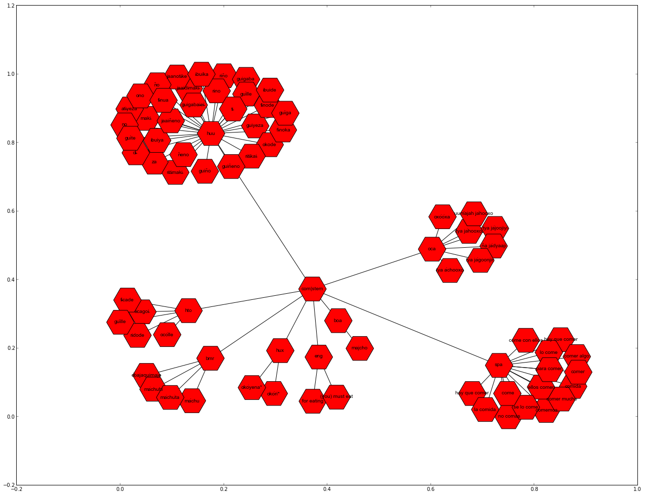
Extract a subgraph for the stem of “comer”
As an example how to further process the graph we will extract the subgraph for the stem “comer” now. For this the graph is traversed again until the node “com|stem” is found. All the neighbours of this node are copied to a new graph. We will also remove the sources from the node strings to make the final visualization more readable:
In[66]:
comer_graph = networkx.Graph()
for node in combined_graph_stemmed:
    if node == "com|stem":
        comer_graph.add_node(node)
        # spanish nodes
        comer_graph.add_node("spa")
        comer_graph.add_edge(node, "spa")

        for sp in combined_graph_stemmed[node]:
            if "lang" in combined_graph_stemmed.node[sp] and combined_graph_stemmed.node[sp]["lang"] == "spa":
                comer_graph.add_node(sp)
                comer_graph.add_edge("spa", sp)

                for n in combined_graph_stemmed[sp]:
                    if ("lang" in combined_graph_stemmed.node[n] and combined_graph_stemmed.node[n]["lang"] != "spa") and \
                            ("is_stem" not in combined_graph_stemmed.node[n] or not combined_graph_stemmed.node[n]["is_stem"]):
                        s = n.split("|")[0]
                        lang = combined_graph_stemmed.node[n]["lang"]
                        comer_graph.add_node(lang)
                        comer_graph.add_edge(node, lang)
                        comer_graph.add_node(s)
                        comer_graph.add_edge(lang, s)
Plot the subgraph with matplotlib
The subgraph that was extracted can now be plotted with matplotlib:
In[67]:
import matplotlib.pyplot as plt
fig = plt.figure(figsize(22,17))
networkx.draw_networkx(comer_graph, font_family="Arial", font_size=10, node_size=3000, node_shape="H")
Export the subgraph as JSON data
Another method to visualize the graph is the D3 Javascript
library. For this we need to export the graph as
JSON data that will be loaded by a HTML document. The networkx contains
a networkx.readwrite.json_graph module that allows us to easily
transform the graph into a JSON document:
In[68]:
from networkx.readwrite import json_graph
comer_json = json_graph.node_link_data(comer_graph)
The JSON data structure can now be written to a file with the help of the
Python json module:
In[69]:
import json
json.dump(comer_json, codecs.open("swadesh_data.json", "w", "utf-8"))
An example HTML file to visualize with D3 is here: